8 Splines

Polynomials are a natural place to begin for interpolation; they’re simple functions, and we already have some familiarity with approximating functions by Taylor polynomials (the study of which took us right to calculus/analysis!). As we saw, there’s a natural linear algebraic interpretation, which makes for a conceptually clean theory of interpolation by choosing different bases, like the Newton basis (fast evaluation) and the Lagrange basis (easy to write down). However, these interpolations have some undesireable features.

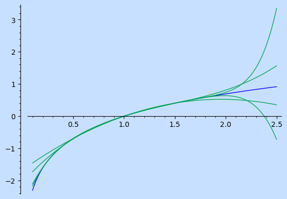
Consider, for example, a couple polynomial interpolations of the natural logarithm on the interval \((0,2)\) with evenly spaced nodes.

The interpolation improves as the number of nodes increases. However, notice that the behavior toward the endpoints is pretty erratic. In fact, adding a single extra node anywhere will cause the function to switch from even to odd (or the reverse). One can induce a fairly dramatic change near \(2\) by adding a single extra point at the opposite end of the interval, even if that point is extremely close to one that’s already being interpolated. The problem is even worse over a larger interval. We would like a way of interpolating that keeps change local.

8.1 Polynomial Splines

Since we like polynomials, though, we will still use them, but rather than stretching a single polynomial to cover the entire interval, we will use many polynomials and produce a piecewise polynomial interpolation. As you likely remember from calculus, piecewise functions have a couple issues: they tend not to be continuous across pieces. Even a continuous piecewise function, like the absolute value, may not be differentiable. Splines are:

piecewise (to keep changes local),
polynomials (simple functions, ultimately we can solve for some coefficients with linear algebra),
continuous, even differentiable (smoother appearance).

The complete definition is as follows.

Definition 8.1 Let \((x_0,y_0),...,(x_n,y_n)\) be some points with \(x_0 < x_1 < ... < x_n\). As usual, \(x_i\) values are called nodes (knots, in other places). Those with \(0 < i < n\) are called inner nodes.

Then a degree \(d\) spline interpolating these points is a piecewise function \(S\) on the interval \([x_0,x_n]\) such that:

The domains of its piecewise components are the intervals \(I_i = [x_{i-1},x_{i})\) for \(1\leq i < n\) along with \(I_n = [x_{n-1},x_n]\),
On each \(I_i\), \(S\) is given by a polynomial \(P_i\) of degree at most \(d\),
At each inner node \(x_i\), \(S\) is \(d-1\)-times continuously differentiable. Equivalently, \[ P_i^{(k)} (x_i) = P_{i+1}^{(k)}(x_i)\] for \(0\leq k \leq d\). This is called the spline condition.

For example, a degree \(0\) spline is piecewise constant – the spline condition is vacuous, so it isn’t even continuous. A degree \(1\) spline is just the union of the line segments connecting consecutive points, so it is continuous but usually not differentiable. A degree \(2\) spline is continuous and continuously once-differentiable.

Theorem 8.1 Given \(n\) nodes \(x_0<...<x_n\), the space \(\mathcal P\mathcal P_d\) of piecewise polynomial functions of degree at most \(d\) has dimension \(n(d+1)\).

The space \(\mathcal S_d\) of degree \(d\) splines is a subspace of \(\mathcal P\mathcal P_d\) and has dimension \(n+d\). Given values \(y_0,...,y_n\), the set of splines interpolating \((x_i,y_i)\) is an affine subspace of dimension \(d-1\).

Proof. It is easy to see these are vector spaces. Scalar multiplication and addition preserve the spline condition.

For \(\mathcal P\mathcal P\), it is easy to check that it has as a basis the monomials of degree at most \(d\) restricted to each piece. There are \(n\) pieces and \(d+1\) monomials on each. Or, in other words, \(\mathcal P\mathcal P_d\) is a direct sum of \(n\) copies of \(\mathcal P_d\), the isomorphism given by restriction and addition.

Note that the map \(\phi_{k,i}: \mathcal P_d \to K\) given by \(p \mapsto p^{(k)}(x_i)\) is linear. The spline condition insists that for each \(0<i<n\), the \(d\) maps \(\phi_{k,i}\) for \(0\leq k \leq d-1\) agree on the consecutive copies of \(\mathcal P_d\) in the direct sum. This imposes a total of \(d(n-1)\) independent linear conditions on \(\mathcal P\mathcal P\) which are satisfied precisely by the splines. Therefore, \(\mathcal S_d\) has dimension \[n(d+1)-d(n-1) = n + d.\]

Finally, observe that interpolation imposes further (affine) conditions on the value of \(\phi_{0,i}\) at each node. There are \(n+1\) of these conditions, all independent, and so the homogenous solution space is cut down to dimension \(n+d-(n+1) = d-1\).

Concretely, for each inner node \(x_i\), take the polynomial pieces \(P(x)\) and \(Q(x)\) to either side one and write them as \(\sum a_i (x-x_i)^i\) and \(\sum b_i(x-x_i)^i\). The spline condition requires \(a_i=b_i\) for \(i\leq d-1\), while interpolation means \(a_i=b_i = y_i\). These conditions leave the \(d+1\) top degree terms free and the two extra interpolation conditions at the endpoints cut the dimension down to \(d+1-2 = d-1\).

It is worth noting that there are many variations on splines. Common ones include specifying different degrees on different intervals, and a different number of agreeing derivatives at the nodes; if you know your function is basically linear on an interval, there may not be much value in using a high degree polynomial there, and then you may not want this line to impose strong conditions on higher derivatives of its neighbors. Also, splines can be built out of functions other than polynomials. For example, Bézier splines, common in graphic design, are built from parametric functions called Bézier curves.

8.2 Natural Cubic Splines

Among the polynomial splines, the degree three cubic splines are especially common. Theorem 8.1 tells us this interpolation problem has two degrees of freedom, which is often dealt with as follows.

Definition 8.2 A natural cubic spline is a degree \(3\) spline with endpoints \(x_0,x_n\) subject to the further condition \(S''(x_0) = S''(x_n) = 0\). This is called the naturality condition.

There is a unique natural cubic spline interpolating \((x_0,y_0),...,(x_n,y_n)\).

The spline and naturality conditions give rise to a well-structured interpolation problem.

Given points \((x_0,y_0),...,(x_n,y_n)\), the natural cubic spline \(S\) interpolating them can be found as follows.

As usual, let \(P_i\) be the polynomial on the \(i\)th interval. Let \(c_i = S''(x_i)\). Since \(P_i\) is cubic, \(P_i''\) is linear, and we know that \(P_i''(x_{i-1}) = c_{i-1}\) and \(P_i''(x_i) = c_i\) by the second derivative piece of the spline condition. This identifies it as the line \[P_i''(x) = \frac{x-x_{i-1}}{x_i-x_{i-1}}c_i - \frac{x-x_i}{x_i - x_{i-1}} c_{i-1}.\]

A second antiderivative of this is \[P_i(x) = \frac 1 6 \frac{(x-x_{i-1})^2}{x_i-x_{i-1}} c_i - \frac 1 6 \frac{(x-x_i)^2}{x_i-x_{i-1}} c_{i-1} + C_i(x-x_i) + C_i'(x-x_{i-1}).\] since its second derivative is \(P_i''\) and it forms a vector space of the right dimension.

The interpolation conditions require \[C_i = \frac{y_{i-1}}{x_{i-1}-x_i} - \frac{c_{i-1}(x_{i-1}+x_i)}{6}\] \[C_i' = \frac{y_i}{x_i-x_{i-1}} - \frac{c_i(x_i+x_{i-1})}{6}\] (note the difference of squares).

Therefore, once we know the \(c_i\) we’ll have the \(P_i\). These will come from the compatibility of the first derivatives, so look at \[P_i'(x) = \frac {c_{i-1}} 2 (x-x_i) + \frac {c_i} 2 (x-x_{i-1}) + C_i + C_i'\]

From \(P_i'(x_i) = P_{i+1}'(x_i)\) as well as \(P_0''(x_0) = 0\) and \(P_n''(x_n) = 0\) and a bit of algebra, we will obtain the following system of equations \[\begin{bmatrix} D_1 & d_2 & 0 \\ d_2 & D_2 & d_3 & 0\\ 0 & d_3 & D_3 & d_4 & 0 \\ & \ddots & \ddots & \ddots & \ddots & \ddots \\ & & 0 & d_{n-3} & D_{n-3} & d_{n-2} & 0 \\ &&& 0 & d_{n-2} & D_{n-2} & d_{n-1} \\ &&&& 0 & d_{n-1} & D_{n-1} \end{bmatrix} \begin{bmatrix} c_1 \\ c_2 \\ c_3 \\ ... \\ c_{n-3} \\ c_{n-2} \\ c_{n-1} \end{bmatrix} = \begin{bmatrix} y''_1 \\ y''_2 \\ y''_3 \\ ... \\ y''_{n-3} \\ y''_{n-2} \\ y''_{n-1} \end{bmatrix}\]

where: \[\begin{align*} d_i &= x_i - x_{i-1}\\ D_i &= 2(d_i + d_{i+1})\\ y_i'' &= 6\frac{y_{i+1} - y_i}{x_{i+1} - x_i} - 6\frac{y_i - y_{i-1}}{x_i - x_{i-1}} \end{align*}\] (it’s no accident that this looks a little like divided differences)

This matrix has some really nice features:

nonnegative entries,
strictly diagonally dominant,
tridiagonal,
symmetric.

These guarantee good behavior for pretty much any numerical method. Row reduction will be quick and straightforward, and even pivoting is unnecessary.

With the work of the previous sections in mind, it’s likely you’re already wondering about adjusting polynomials into a form which can be evaluated more quickly. This would look like \[P_{i+1}(x) = y_i + (x-x_i) \biggl( C_i + (x-x_i) \bigl( B_i + (x-x_i) A_i \bigr) \biggr).\]

One can show that the coefficients are

\[\begin{align*} A_i &= \frac 16 \frac{c_i - c_{i-1}}{t_i - t_{i-1}},\\ B_i &= \frac{c_{i-1}}{2},\\ C_i &= \frac{y_i - y_{i-1}}{t_i - t_{i-1}} - \frac 16 (t_i - t_{i-1})(2c_{i-1} - c_i), \end{align*}\]

for \(0 < i < n\).

8.3 \(B\)-Splines

Implementing these algorithms isn’t particularly illuminating. The built-in functions are easy to use:

points = [(2*i/8,log(2*i/8)) for i in range(1,9)]
S = spline(points)
show(S(1.1))

\(\displaystyle 0.09602853016726794\)

Sage ultimately uses the GSL spline implementation. As we saw when studying polynomials, a good choice of basis can be quite helpful. The GSL library uses what are called \(B\)-splines. For a fixed infinite collection of nodes, they are defined inductively.

Definition 8.3 Given nodes \(... < x_{-1} < x_0<x_1<...\), the \(B\)-splines of degree \(0\) are \[B_i^0(x) = \begin{cases} 1 & x_i \leq x < x_{i+1}\\ 0 & \textrm{otherwise} \end{cases}\] and the \(B\)-splines \(B^k_i\) of degree \(k\) are inductively defined by \[B_i^k(x) = \frac{x-x_i}{x_{i+k} - x_i} B^{k-1}_i(x) + \frac{x_{i+k+1} - x}{x_{i+k+1} - x_{i+1}}B_{i+1}^{k-1}(x)\]

The construction ensures that \(B_i^k\) is a polynomial of degree \(k\). This definition is quite a lot like the homotopy version of polynomial interpolation discussed previously: \(B_i^k\) is something like a weighted average of \(B^{k-1}_i\) and \(B_{i+1}^{k-1}\). By inspection, we see that \(\sum B_i^0\) is the constant \(1\). In fact, this is true in higher degree too,

Theorem 8.2 The \(B\)-splines of degree \(k\) sum to the constant \(1\): \[\sum_{-\infty}^\infty B_i^k(x) = 1\] for all \(x\).

Proof. For simplicity, we assume the nodes are integers, so \(x_i = i\). The general result has a similar but more notationally messy proof. The definition simplifies to \[B_i^k(x) = \frac{x-i}{k} B^{k-1}_i(x) + \frac{i+k+1 - x}{k}B_{i+1}^{k-1}(x)\] Notice that this means \(B_{i+1}^k(x) = B_i^k(x-1)\). This translation property is messier in the general situation.

We can prove by induction that \[\frac d{dx} B_i^k(x) = B_i^{k-1}(x) - B_{i+1}^{k-1}(x).\] By direct calculation, we first get \[\frac d{dx} B_i^k(x) = B_i^{k-1}(x) - B_{i+1}^{k-1}(x) + \frac {x-i}{k} \frac d{dx} B^{k-1}_i(x) - \frac{i+k+1-x}{k}\frac d{dx}B_{i+1}^{k-1}(x),\] and our translation observation tells us \(B_{i+1}^k(x) = B_i^k(x-1)\), while induction and a similar substitution show that the last two terms vanish.

Now we are essentially done. Note that \(B_i^k\) is zero outside \([i,i+k+1]\), so only finitely many terms of the following sum are nonzero in a neighborhood of any given \(x\). This means there are no convergence issues to consider.

So, by induction, we get \[\begin{align*} \frac d{dx}\sum_{-\infty}^\infty B_i^k(x) &= \sum_{-\infty}^\infty B_i^{k-1}(x) - B_i^{k-1}(x-1)\\ &= \sum_{-\infty}^\infty B_i^{k-1}(x) - \sum_{-\infty}^\infty B_i^{k-1}(x-1)\\ &= 1-1\\ &= 0 \end{align*}\]

Therefore, the sum is constant, and hence can be determined by evaluating it at any point, such as \(x=0\). \[\begin{align*} \sum_{i=0}^\infty B_i^k(0) &= \sum_{-\infty}^\infty \frac{0-i}{k} B^{k-1}_i(0) + \frac{i+k+1 - 0}{k}B_{i+1}^{k-1}(0)\\ &= \sum_{-\infty}^\infty \frac{-i}{k} B^{k-1}_i(0) + \frac{i+1}{k}B_{i+1}^{k-1}(0) + B_{i+1}^{k-1}\\ &= -\sum_{-\infty}^\infty \frac{i}{k} B^{k-1}_i(0) + \sum_{-\infty}^\infty \frac{i+1}{k}B_{i+1}^{k-1}(0) + \sum_{-\infty}^\infty B_{i+1}^{k-1} \end{align*}\]

The first and second terms cancel, since they’re the same sum (but for a shifted index) with opposite signs. The last is \(1\) by induction.

The well-controlled supports of \(B\)-splines mean that the linear algebra problem associated to interpolating with them is quite simple and (retroactively) anticipates our tridiagonal matrix above. Form the infinite matrix \(A = [B_i^k(x_j)]_{i,j}\) representing the evaluation map, and notice that since \(B_i\) is zero outside \([x_i,x_{i+k+1}]\) the entries are all zero away from \(k\) “diagonals”. We can truncate it to a square of interest that includes the finitely many nodes we’re interested in, and solve the associated system of equations.

Exercises

Exercise 8.1 Determine whether the following is a quadratic spline: \[f(x) = \begin{cases} (x+2)^2 - 18(x+2) + 20 & x< -2\\ 4x^2 - 2x& -2\leq x \leq 2\\ 3(x-2)^2 + 4(x-2) + 12 & x > 2 \end{cases}\]

Exercise 8.2 Determine whether the following is a natural cubic spline: \[f(x) = \begin{cases} 1 - 2x^2 - \frac 1 2 (x^3 -8x) & -2\leq x \leq -1\\ x^2 + 2 + \frac 1 3 (2x^3 + x) & -1\leq x \leq 0\\ x^2 + 2 - \frac 1 3 (x^3 + x) & 0\leq x \leq 1 \end{cases}\]

Exercise 8.3 Find coefficients \(a,b,c,d\), which make the following a cubic spline: \[f(x) = \begin{cases} x^3 & -1\leq x \leq 0\\ a+bx+cx^2 + dx^3 & 0\leq x \leq 1 \end{cases}.\]

Then try with \[f(x) = \begin{cases} x^3 & 0\leq x \leq 1\\ a+bx+cx^2 + dx^3 & 1\leq x \leq 2 \end{cases}.\]

Exercise 8.4 Determine a quadratic spline approximation to \(f(x) = \arctan(x)\) with nodes \(x=-1,0,1\).

Exercise 8.5

Let \((x_0,y_0),...,(x_n,y_n)\) be some points to interpolate. Find a degree \(d\) and degree \(d\) spline \(S\) such that \(S\) is a degree \(D\) spline for all \(D \geq d\).
What do you expect to happen when \(n >> d\) and a degree \(d\) spline also a degree \(d+1\) spline? What if \(n << d\)?

Exercise 8.6 Let \(S\) be a degree \(d\) spline.

Show that the derivative \(S'\) is a degree \(d-1\) spline with the same nodes.
Given a spline \(S\) and point \(a\) in its domain, show that the integral \[\int_a^x S(t) dt\] is a degree \(d+1\) spline with the same nodes.

Exercise 8.7 Using Exercise 8.6, give a different (and somewhat more rigorous) proof of Theorem 8.1 by induction on degree, starting from the observation that the degree \(0\) splines are exactly the piecewise constant functions, which have dimension \(n\).